

How to Distribute Leverage and Lot Sizing Between Trades

You may be lucky enough to find or create more than one good system, but the extra challenge you will confront is, how do you weigh and distribute the leverage and lot sizing between the different systems to stay within sound money management principles?
Find out in this article how to properly distribute the leverage and lot sizing between the different trading systems to stay within sound money management principles.
Table of Contents
As we have seen, it is smart leverage practice to trade no more than 2:1 leverage per trade (or 2% Equity Risk), which is akin to trading 1 mini lot per $5000, or 1 micro lot per $500. But what if you were trading with more than one strategy, and consequently you have several concurrent trades open from different systems working on the same or different currency pairs?
You might think you are diversified when in fact the net correlation between the different systems is so great that your aggregate risk is not reduced but magnified.
This article will try to gauge how you can measure the degree of difference between pairs and strategies in order to assign increased leverage/risk to the difference.
Every portfolio of strategies will start with a baseline of 2:1 leverage in aggregate. In my %Equity Risk formula, 2:1 leverage is akin to 2% risk, or 0.02. If I have two strategies I will divide 2% by 2 to get 1% risk per strategy, and if I have five strategies I will divide 2% by 5 to get 0.4% risk per strategy. However, I will be able to increase the baseline 2% aggregate Risk based on measured degrees of market and behavioral difference between strategies.
For instance, if I have two strategies trading on completely uncorrelated pairs, such as EURUSD and AUDNZD, I can award 1% extra risk to the portfolio to make it an aggregate risk of 3% and thus trade 1.50% for each strategy.
Let us now examine three areas where diversification, correlation, and difference can be measured and awarded:
- Market Diversification: Diversifying into uncorrelated pairs
- Behavioral Diversification: Diversifying into differences in strategy logic, time frame, duration and trade frequency
- Profitability Diversification: Diversifying into differences in profitability and robustness.
Market Diversification
You have all heard of the adage, “Don’t put all your eggs in the same basket” and what this is popularly taken to mean is that you don’t put all your money in one asset class (savings and CD accounts, stocks, bonds, real estate, commodities, foreign currency, etc.) or one instrument within the class, but instead, you aim to diversify your investment into multiple asset classes and different types of instruments.
The argument put forward to diversify into multiple asset classes is a sound one: when things go bad, your entire portfolio does not have to go down the tubes. While stocks and real estate declined during the last recession, precious metals like gold and silver quickly recovered from their fall and outperformed almost every other class during the recovery phase, and so having something from each class (along with keeping money in super-safe savings and CDs) can soften the blow when things go south.
The argument put forward to diversify into different types of instruments is usually found in the world of stocks: if you put all your money into similar stocks you could end up losing a good part of it when that sector deteriorates for whatever reason.
We saw how the internet stocks got hammered in 2001 after the bursting of the Dot Com Bubble (1995-2000), and then we saw how the bank stocks were almost wiped out in 2008 after the bursting of the US Housing Bubble (2002-2007). These are good lessons. If one is investing in the world of stocks, one should focus on several sectors (banking, utilities, healthcare, tech, and consumer goods) and find the best representative companies from each.
That being said, it is not uncommon for all sector stocks to dramatically fall in lockstep after the bursting of an asset bubble. In periods of uncertainty or crisis, markets tend to perform together.
Though Forex does not have specialized sectors like the world of stocks, it does have regional sectors that have distinct economic fundamentals that set themselves apart from other regions. Below is a table grouping currencies according to the region:
| Region | Popular Currencies within Each Region | Notes |
|---|---|---|
| North America | US Dollar (USD), Canadian Dollar (CAD), Mexican Peso (MXN) | US Dollar is the king currency |
| South America | Brazilian Real (BRN), Argentina Peso (ARS), Colombian Peso (COP) | Hard to find at any FX Brokerages |
| Western Europe | British Pound (GBP), Euro (EUR), Swiss Franc (CHF), Danish Krone (DKK), Norwegian Krona (NOK), Swedish Krona (SEK) | There is high correlation between CHF, DKK, NOK, and SEK. Scandinavian currencies are traded at few FX Brokerages. |
| Eastern Europe | Czech Koruna (CZK), Hungary Forint (HUF), Poland Zloty (PLN), Turkish Lira (TRY) | Eastern European Currencies are traded at few FX Brokerages |
| Middle East | Qatari Rial (QAR), Kuwaiti Dinar (KWD), UAE Dirham (AED), Saudi Riyal (SAR), | Middle Eastern Currencies are traded at few FX Brokerages |
| Africa | South African Rand (ZAR) | ZAR is traded at few FX Brokerages. |
| Oceana | Australian Dollar (AUD), New Zealand Dollar (NZD) | Very correlated |
| East Asia | Japanese Yen (JPY), Chinese Yuan Renminbi (CNY), Hong Dollar (HKD), Malaysian Ringgit (MYR), Singapore Dollar (SGD), | Only JPY is found at FX Brokerages; JPY stands as a proxy currency for East Asia |
| South Asia | Indian Rupee (INR), Pakistan Rupee (PKR) | Found at few FX Brokerages. |
While it seems that there are nine regions one can diversify one’s currency investments into, most FX Brokerages only offer currencies in four of them: North America, Western Europe, Oceana, and East Asia (and of East Asia, only JPY). Few FX brokerages offer currencies from all regions, which limits one’s ability to diversify according to regional economic differences.
Moreover, there is no guarantee that spreading your risk across multiple currencies from different regions can protect you from capital market risk; for instance, during the 2008 financial crisis and resulting panic, most currencies from most regions depreciated close to 25%, while only the USD and JPY grew in value. As I have said before, in periods of uncertainty or crisis, markets tend to perform together. The only sure insurance from market risk is to limit one’s exposure to any one currency, and don’t hold on to any currency like an investment but instead trade it short term.
Moving over the technical side, it can be advantageous to select more than one pair to trade for three reasons:
- A currency pair can sometimes get stuck in a small trading range, making it difficult to trade, while other pairs might be making trends;
- Following more than one pair increases the odds that a profitable trend will not be missed;
- Diversification, especially when the pairs are not correlated, can reduce risk.
It is this last point, uncorrelated diversification can reduce risk, that we will focus our attention upon.
Risk is both correlated and uncorrelated. Correlated risk cannot be eliminated through diversification. For instance, if you have trend following strategy worked out on EURUSD, and another trend following strategy worked out on EURCAD, there will be so much correlation between the two pairs that you will most likely enter and exit the respective trends at the same time and in the same direction, thus exposing you to double the risk if the trend fails.
Correlated Risk: The degree of similar movement between pairs.
Uncorrelated Risk: The degree of dissimilar movement between pairs.
The problem with correlated risk is that if you set out to grant 2:1 leverage per trade across all the correlated pairs, you are greatly magnifying your leverage and risk. We are more interested in discovering the uncorrelated differences between pairs.
Measuring the Uncorrelated Differences Between Pairs
You can turn to visually examine the currencies charts and time frame you are interested in trading and get a rough idea of how pairs follow or depart from each other.
Or you can turn to different websites calculate the correlation percentage between different pairs on different time frames:
Each website has its respective advantages. An interesting view has Investing.com for the all-at-once visual correlation between 29 pairs on selected time frame and period, which would be daily and 200 or 300 period. Smaller time frames and periods highlights the deviance more acutely, but I am interested mostly in the big picture. Bear in mind that correlations do not remain constant, and so choosing two pairs that seem uncorrelated in the last year may surprise you in being far more correlated in coming months.
If interested in diversifying outside of the EUR/USD, select EUR/USD against 29 pairs on Daily 300 Period (on Aug 24, 2012):
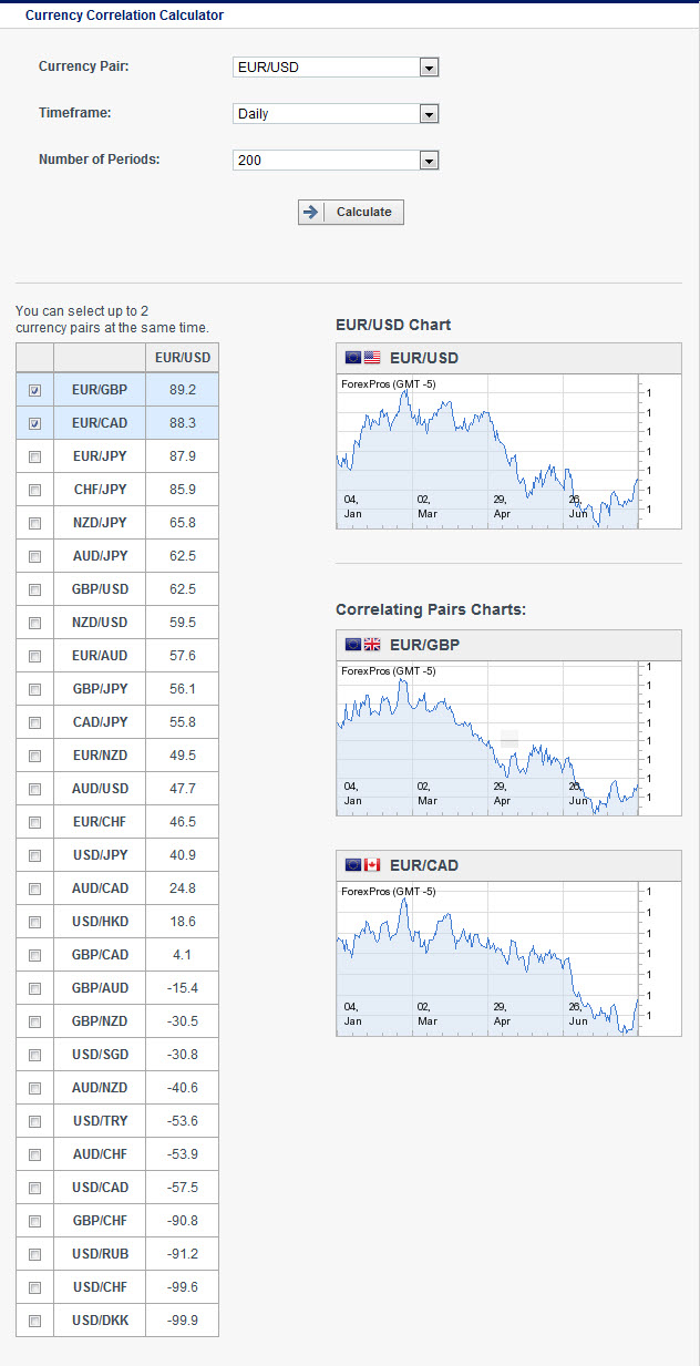
Assuming that anything above +70% (or below -70%) is fairly correlated, it seems that our list of 29 pairs can be reduced to 21 non-correlated pairs. Does that make sense? The first four pairs (EUR/GBP, EUR/CAD, EUR/JPY, CHF/JPY) all have greater than 70% correlation, and likewise, the last four pairs (USD/DKK, USD/CHF, USD/RUB, GBP/CHF) all greater than -70% correlation. If you are going to trade your trend following strategies on uncorrelated pairs, you would be forced to choose the 21 in the middle, and then conduct a correlation analysis on each of them, to see what degree of correlation they have with each other.
But you don’t have to select pairs based only on their non-correlatedness or eliminate pairs because of their higher, historical correlation. Instead, you can use the correlation percentiles as a way of measuring up and rewarding more risk to your aggregate risk, in the following formula:
First, we have to select a pair that will act as the standard of comparison. You can pick EUR/USD because its popularity and liquidity make it ideally suited for trading trends. Next, turn to the correlation table above and select three additional strategies that are uncorrelated, such as AUD/JPY (62.5), GBP/USD (62.5), AUD/USD (47.7), providing that back-test performance is strong on all three pairs. From each of these extract the percentile of non-correlation (e.g., GBP/USD has a non-correlation of 37.5%, or 0.375).
Currency Pairs: 4
AUD/JPY Non-Cor%/1000: 0.375 / 100 = 0.00375
GBP/USD Non-Cor%/1000: 0.375 / 100 = 0.00375
AUD/USD Non-Cor%/1000: 0.523 / 100 = 0.00523BaselineRisk% + Uncorrelated%/100 / CurrencyPairs(0.02 + 0.00375+0.00375+00523)/ 4
= 0.0081 (0.8%) risk per strategy
Notice how we did not simply grant 2% risk for each uncorrelated pair. That would allow Mr. Market to teach you a hard lesson, namely that no matter how uncorrelated you think different pairs can be, they do often travel together, particularly in periods of uncertainty or crisis.
Instead of carrying 2% risk for each pair, which would give us an over-leveraged aggregate risk of 8%, or instead of dividing 2% by the number of pairs, which would give us an under-leveraged per strategy risk of 0.5%, we instead add a bit more risk % to the 2% baseline based on measured differences, which in the above example calculation gives us a more reasonable 0.8% risk per strategy.
Alternate Approach to Measuring and Awarding Correlation:
It is possible to forego the correlation matrix itself and just assume that all major pairs (and yen crosses) have a roughly 20% uncorrelated factor. Thus, if you were to trade the trend following strategy on 5 currency pairs, then you could effectively add 1% (0.002 * 5) to your original 2% Risk to get 3%, and then divide by 5, to get at 0.6% for each pair.
Complication: One further complication in the subject of currency pair correlations is that often a lead-lag relationship occurs that is invisible to the system tester, and most correlations themselves change over time. Efficient diversification is thus a useful and important subject but not a simple one.
Behavioral Diversification
So far in the above, we have mostly confined to talking about how one can measure and award greater risk to the degree of non-correlation detected between pairs. But what about measuring and awarding greater risk to the degree of non-correlation detected in the differences between strategies?
For instance, we know that there is a major difference between an MA Cross trend following strategy and an RSI Overbought/Oversold, counter-trend strategy, and we have to account for that difference. Herein we have to rely less on statistical, quantifiable differences, as what we discovered from a correlation table, and more on observable, qualitative differences.
There are basically three behavioral differences between strategies:
| Behavioral Difference | Description | Measured Differences |
|---|---|---|
| Type | 1. Trending Following A. Indicator Crossover B. Breakout from Support/Resistance2. Counter-Trend A. Indicator Crossover (Oversold/Overbought or Upper/Lower Band) B. Bounce from Support/Resistance | We would assign a 100% difference between the two opposing strategy types, and a 30% difference between A and B within the same strategy type. |
| Time Frame | There are 9-time frames a strategy can be worked out upon: M1, M5, M15, M30, H1, H4, D1, W1, M1. | We would award 10% difference for each difference in a time frame. If you had a strategy worked out on the D1 time frame, and the same strategy type worked out on the M30 time frame, we would estimate a 30% difference between the two. |
| Frequency | You have to figure upon the number of trades per month for each strategy and account for the difference. | We would award 1% for each trade per month difference. For instance, if one strategy were to give out 10 trades per month, and the other strategy was to give out 30 trades per month, we would assign 20% difference between the two (20X1%). |
How would I factor in the measured degree of non-correlation between strategies into risk formula?
The formula would be:
For instance, suppose one has a MACross trend following strategy worked out on a H4 chart that trades 10 times per month, and a RSI Counter trend strategy worked out on a M15 chart that trades 30 times per month.
Then award the following percentiles:
Difference in Type: 100%, or 0.10 / 100 = 0.01
Difference in Time Frame: 3 time frames apart, or 0.30 / 100 = 0.003
Difference in Frequency: 20 trades per month, or 0.20 /100 = 0.002(BaseRisk% + UnCorrelated%/100) / Currency Pairs or Strategies0.02 + 0.01 + 0.003 + 0.002 / 2
= 0.387 / 2 = 0.0193 (or 1.93%) per strategy
Now, what if the trend following strategy was working on EUR/USD and the counter trend was working on GBP/USD, then you can add 0.00375 to the aggregate risk before dividing by 2:
Difference in Pair: 37.5%, or 0.375/100 = 0.00375Difference in Type: 100%, or 0.10 / 100 = 0.01
Difference in Time Frame: 3 time frames apart, or 0.30 / 100 = 0.003
Difference in Frequency: 20 trades per month, or 0.20 /100 = 0.002(BaseRisk% + UnCorrelated%/100) / Currency Pairs or Strategies0.02 + 0.00375+ 0.01 + 0.003 + 0.002 / 2
=0.424 /2 = 0.21 (or 2.1%) per strategy
If you are comparing more than two strategies, it is easier to compare all additional strategies against your principal strategy and measure/aware the differences. Keep in mind that we have assigned estimated percentiles based on estimated differences, and you are free add or subtract or completely change the method of measuring and awarding based on different observations of your own. There is no clear rule for how to go about doing it, and so we making a rudimentary stab of our own.
Note: Ten losing trades in different markets is the same as ten consecutive losses in one market. The drawdown is the same. Thus, diversification can bring problems as well as reduce risk. The frequency of trading in different markets will increase the risk of a series of losses across markets.
Profitability Weighting
So far, we have figured on how to measure and award the differences between pairs and strategy behaviors, but what about the differences in profitability and robustness between strategies? What if your MACross, trend following strategy on EUR/USD H4 with 10 trades per month had 1.7 profit factor with 50% accuracy, but your RSI counter-trend strategy on GBP/USD M15 with 30 trades per month had a profit factor of 3.0 with 75% accuracy. Clearly, the RSI GBP/USD strategy is far superior and deserves more weighting.
In this case, we can turn to Optimal F to get a more fair base line starting percentage for each strategy. The formula for OptimalF is:
Data for the two scenarios:
PercentWin: 50%Profit Factor: 1.7Optimal F = (0.50 * (1.7+1)-1) / 1.7 *10) = 0.2 * 10
= 2% (our original base line)
Strategy #2: RSI Counter Trend, GU-M15
PercentWin: 75%
Profit Factor: 3.0Optimal F = (0.75 * (3.0 + 1) -1) / 3.0 * 10 = 0.66 * 10
= 6.6% (3 times our original base)
Now how do we work out these different bases with the differences in pair and behavior correlation?
We just start off with the optimal F base number and add in the awarded differences for each strategy.
For instance, for the two strategies:
Optimal F Base Risk: 2%
Difference in Pair: 37.5%, or 0.375/100 = 0.00375
Difference in Type: 70%, or 0.70 / 100 = 0.007
Difference in Time Frame: 3 time frames apart, or 0.30 / 100 = 0.003
Difference in Frequency: 20 trades per month, or 0.20 /100 = 0.002(BaseRisk% + UnCorrelated%/100) / Currency Pairs or Strategies0.02 + 0.00375 + 0.01 + 0.003 + 0.002 / 2
= 0.03875 / 2 = 0.0193 (or 1.93%) for strategy #1
Base Risk: 6.6%
Difference in Pair: 37.5%, or 0.375/100 = 0.00375Difference in Type: 70%, or 0.70 / 100 = 0.007
Difference in Time Frame: 3 time frames apart, or 0.30 / 100 = 0.003
Difference in Frequency: 20 trades per month, or 0.20 /100 = 0.002(BaseRisk% + UnCorrelated%/100) / Currency Pairs or Strategies0.066 + 0.01 + 0.003 + 0.002 / 2
= 0.0847 / 2 = 0.0423 (or 4.23%) for strategy #2
Now you can see how the different starting risk percentages, based on percentage win and profit factor, can be worked out with the risk rewarding scheme based on differences in pair correlation and behavior (type, time frame, frequency). If you like the optimal form of finding the baseline risk, you might want to start with that and then factor in the differences in pair and strategy behavior.
To find the percentage accuracy and profit factor, be sure to back-test your strategies over a sufficient period of time, preferably more than 2 years. You don’t want to curve fit your strategy over a few months to get stellar accuracy and profit factor and then start off your forward test on a live account with over-leveraged strategies based on over-optimization (overoptimizedF).
It is better to err on the side of caution and use a more conservative base line risk for your initial start, and see if your strategies perform in forward test the same as they do in back test before you fully trust the percentage accuracy and profit factor for your determination of Optimal F risk.
Conclusion
Diversification is a complex subject. The complexity has to do with the weighting amount of different pairs or systems in a portfolio, as well as whether their behavior and performance compliments each other or not.
Obviously, if different pair or systems are used, they should not act in concert. Otherwise, they are essentially the same system, and risk has not been diversified away.
What you are ultimately looking for in the match up of different systems and pairs is complimentary differences: how can the differences in pairs and behaviors and performances work to capture the diverse market moves while minimizing risk?
When looking at different currency pairs and/or systems, you will be looking for how the reduction in uncorrelated risk can reduce MDD and enhance rate of return (ROI). The results of a diversified portfolio are often superior to that of any one system.
 Copy Link
 Share on Facebook
 Share on X
 Share by Email